Graphs are everywhere
Take a look the Amazon product page for Where Is My Flying Car? by J. Storrs Hall:
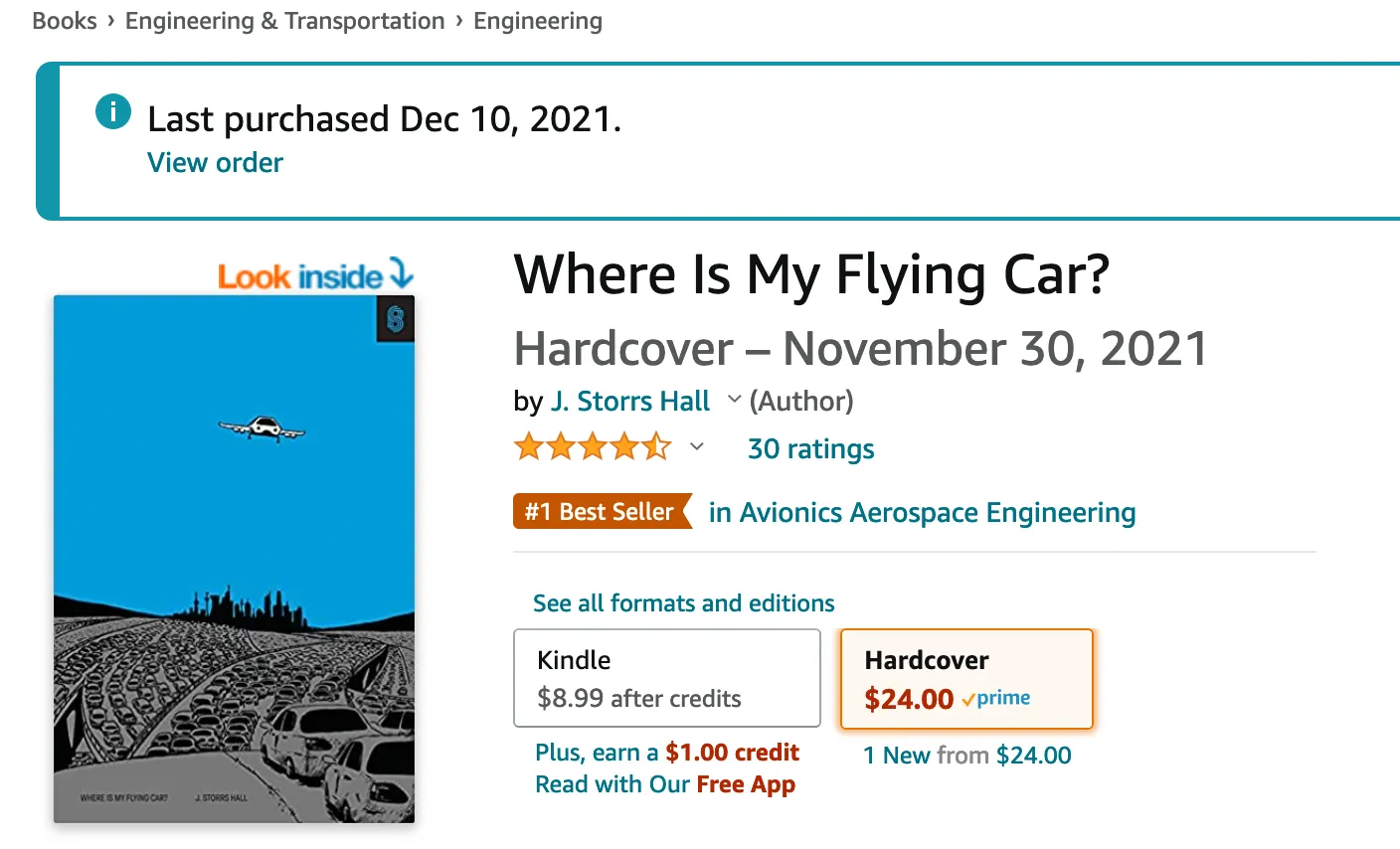
We see the title of the book front and center, but Amazon knows much more about this book than just its title. As we scroll through the page, we see that they also know:
- Who wrote it
- What other books were written by the same author
- What its cover looks like
- What category it belongs to, and where that category lies among the whole hierarchy of categories
- When it was published
- Who published it
- What the publisher says the book is about
- How the publisher describes itself
- How many pages it is
- What formats it’s available in
- Its average star rating
- Who reviewed it and what they said about it.
Look at any major website and you’ll find the same thing: they’re full of entities, like this book on Amazon, and dozens or hundreds of related entities, like authors, reviews, categories, users, dates, tags, and so on.
These entities and the relationships between them form a graph. The websites are often little more than a UI for browsing this graph. That’s sort of the whole point of the web.
The graphs we find on the web are the easiest to see, but all digital environments are graphs. Graphs are the most general data structure, so this isn’t much of an insight. Even hypergraphs can be represented as graphs.
Importantly, all databases represent graphs even if they’re not all graph databases in the specific sense of something like Neo4j. Foreign key relationships in a relational database are graph edges. Documents in a document-oriented database are nodes that have edges to their subdocuments.
So virtually all products or digitial environments of any kind have some kind of graph underlying them. We’ll return to this fact shortly.
Embedding spaces summarize context
Instead of using a graph, there’s another way we can represent our collection of books: as points in space. Instead of talking about what other nodes the book is connected to, what if we said that the book lies at a position in space with coordinates , which we could also write as a vector:
We don’t mean at some position in normal, physical space. We mean in the abstract space of books. Another way to say this is that the book is embedded in space, and another name for the book’s coordinates in this space is its embedding vector.
Like with phsyical space, knowing where something is in abstract book space is only useful if we know where it is relative to other things. In this kind of space, Where Is My Flying Car? would be nearby other similar books like The Great Stagnation by Tyler Cowen (which has a similar topic) and The Dream Machine by M. Mitchel Waldrop (which is by the same publisher). It would be far away from the novel Jitterbug Perfume by Tom Robbins or The Gay Science by Nietzsche, and at some intermediate distance from say How We Learn by Benedict Carey.
Knowing where something is in book space is a substitute for knowing where it is in the graph. We don’t know what other books it has an edge to. Instead, we know what other books are nearby in space, what other books it’s similar to.
What exactly does it mean for two books to be similar? Or, to cut to the chase, what criterion would some algorithm use to determine how similar or dissimilar two things were? Well, that’s up to us. It’s a design decision that depends on what we want to use the similarity metric for.
Say we’re a student trying to understand the history of aviation. Then we’d say that similar books are those that are also about aviation. If instead we we’re Amazon, and we want to build this feature:
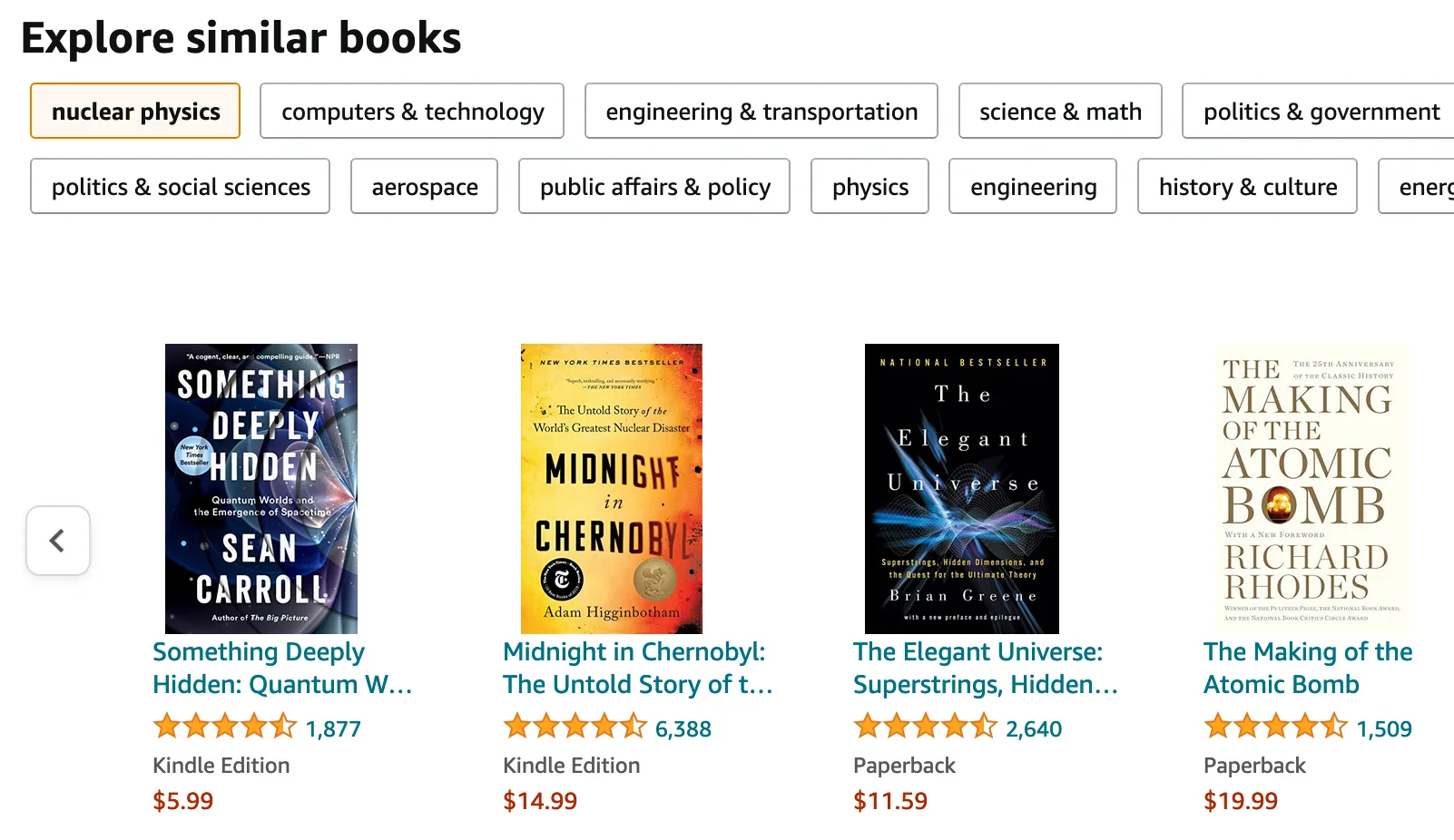
Then the relevant notion of similiarity would be how likely someone who views book is to buy book . Notice that this is quite different, and indeed, none of the books Amazon shows here have anything to do with aviation.
When you look at a whole dataset that has been transformed into this kind of spatial representation, you might see something like this:
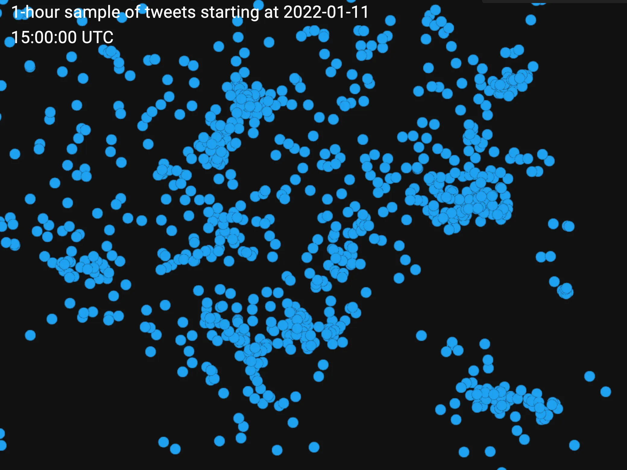
See nebulate.ai for a live demo. The interface is like Google Maps, letting you zoom in and out around the spatial map of the dataset. Each point here is one tweet. They tend to form clusters, clumps of tweets that are about very similar topics. The neighboring clusters tend to be distinct, but still similar, topics. The further out you go, the less similar the tweets are.
This can be a very useful way to visualize a dataset. Since similar points are grouped together, you can more easily browse at the top level, checking a few points in each big cluster to get a general lay of the land and then zooming in on regions you find interesting.
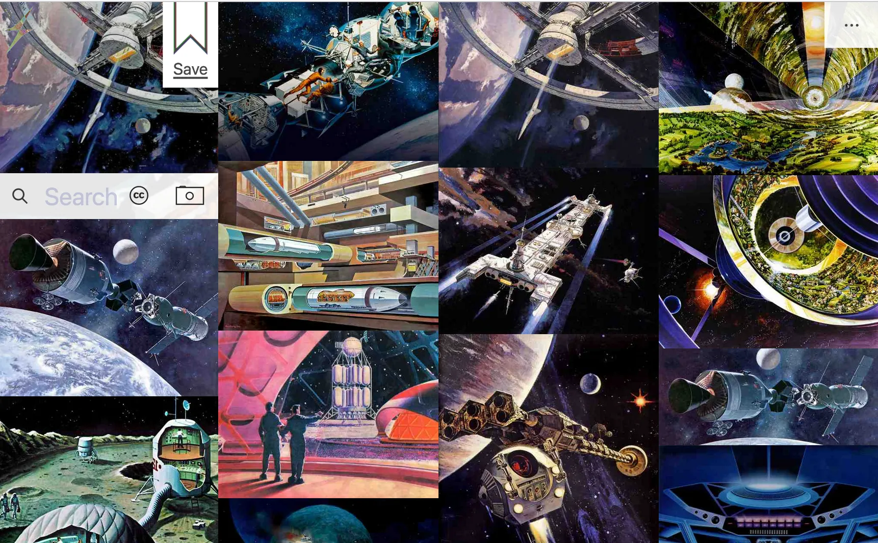
This isn’t only useful for visualization and manual exploration. Being able to retrieve similar pieces of data has many practical applications and can be done very efficiently. We saw Amazon’s similar products feature above, which could implemented this way. There are also many applications in combatting abuse, letting you quickly find other instances of some kind of abusive usage pattern. It can also be a tool for serendipitous creativity as shown by @jbfja’s same.energy, which lets you browse a large collection of images by similarity:
Another useful thing about this embedding space representation is that a piece of data’s embedding vector representation is perfect for feeding into predictive machine learning models.
Let’s say again that you’re Amazon and a new book was added to your catalog, but the publisher didn’t specify what category or genre the book belongs to. You want to have a machine learning model determine this for you. If you start with good embedding representation of the books, it’s much easier for a model to learn to categorize them. It can learn faster and with less labeled data because it can benefit from the same clustering property we saw above. The overall structure of book space has already been worked out. It can assume that books in a similar part of book space will have the same label, so it only needs to learn what label applies to each cluster, which is much easier than learning how to group similar books together from scratch and then also how to label the clusters.
Learning embedding spaces from graphs
But all of this talk of embedding spaces raises an obvious question. How exactly do we compute these embeddings? How do we figure out where to position each book in space?
Well, we train a neural network to do it. It takes the title, author, reviews, and so on as input, and spits out the coordinates for the position in embedding space.
This still doesn’t answer the question. How do we train the network to predict a good embedding for the book? This finally brings us back to where we started. We train the network to predict edges in our graph. Learning to predict good embeddings is a side effect.
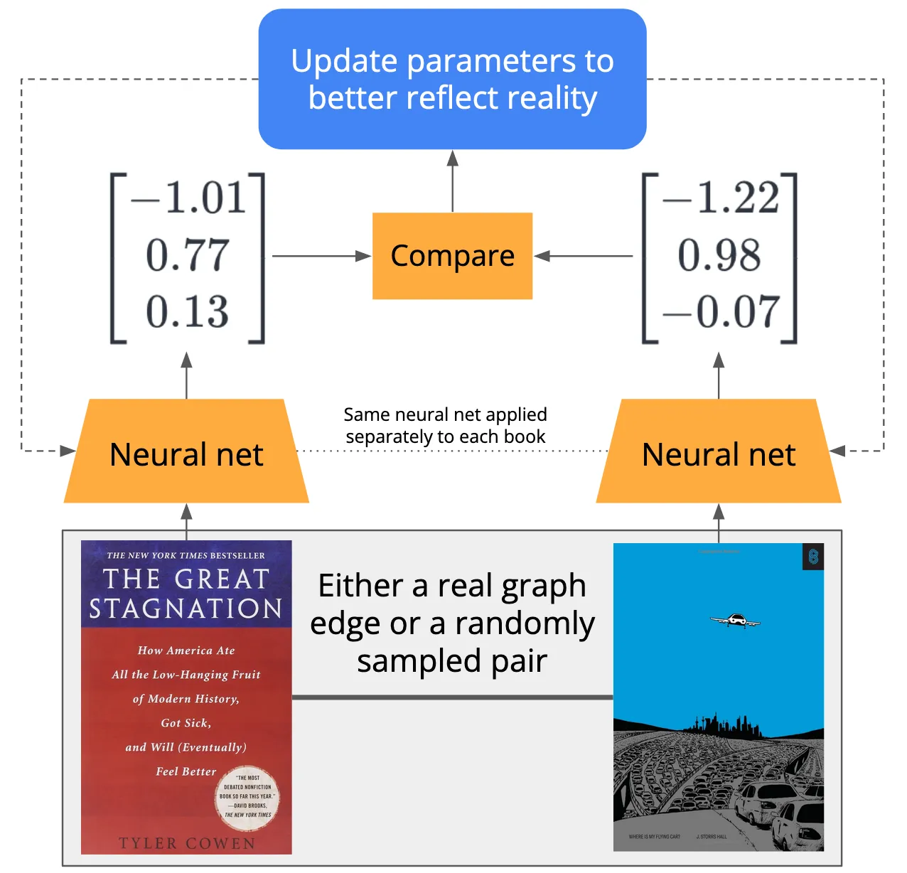
How exactly to do this is an active area of research, but let’s walk through a typical training procedure:
- We sample a book from the catalog.
- With 50% probability, we sample a different book that was also bought by the same user. Otherwise, we sample a random book, which probably has nothing to do with the first.
- We apply our neural network to both books, getting embeddings for each. At first the network is initialized with random parameters, so these won’t be very good embeddings.
- If the two embeddings are close together, we treat this as a prediction that the books were bought by the same person, and if they’re far apart, we treat this as a prediction that they’re a random pair.
- We compare the model’s prediction to the truth, penalizing the model if its prediction disagrees with reality and then update the model’s parameters to make it more likely to be right next time.
- Repeat.
Thinking in terms of the graph, books are nodes, and there is an edge between every pair of books that have been bought by the same person. This task then can be framed as predicting whether there is an edge between a given pair of books.
In order to perform this task well, the model learns to push together books that share an edge and pull apart books that do not. After we let this process run for a while, we end up with a neural network, an embedding model, that generates embedding vectors for books that are close together if the books are similar and far apart if they are not.
Here we chose to train the model on the bought-by-the-same person edges of our graph, but we could have chosen any other kind of edge. If we had trained on written-by-same-author edges, we would then expect books to be embedded such that they are close to the other books written by the same author or by similar authors.
We also could have used both kinds of edges, possibly with different sampling weights, allowing us to choose how much influence we want each kind of edge to have. The way we choose to train the embedding model on our graph is our lever for controlling what kinds of relationships the embedding model will represent. It should depend on what we want to do with the embedding model. Amazon uses the similar books feature to sell more books, so they would likely want to put a lot of weight on bought-by-same-person edges compared to written-by-same-author edges.
Graphs and embeddings: complementary representations
You might be wondering: if we already have the graph, why bother with building the embedding space at all? Why not just run a database query to retrieve the books bought most often bought by people who bought this book? The answer is generalization by way of smoothness.
One way to think about a node in the graph is as a long list of all the edges it might have. In the bought-by-same-person graph, for every book, this list would contain a or a for every other book. If we have books, then for a given book, we’d have a list (usually called a “vector”) that might look like this:
with a total of s and s.
In Amazon’s case, this vector would have millions of entries, and for most books, most of them would be s. We call this kind of vector with many entries and very few non- entries sparse.
This sparse vector representation has the nice property that it is lossless. It’s a complete record of precisely what other books have been bought by the same people who buy this book. We could also say that this representation is discrete — every entry is either or . There’s nothing in between.
Now let’s compare that to the embedding representation. First, a clarification: in this post so far, we’ve been talking about embeddings as coordinates in 3D space. It is possible to use 3 dimensions, but in practice we usually use more, usually between 64 and 1024. While it’s not really practical to visualize such high dimensional spaces directly, all the properties of spatial representations we talked about above still hold. You can still find the distance between points, and these distances correspond to similarity. If we do want to visualize the points in say a 256-dimensional space, there are good ways to first project those points down to 2 or 3 dimensions where they’re easy to visualize.
We say that these embedding vectors are dense. While we usually use more than 3 dimensions, we never use millions of dimensions like the sparse vector representation. The number of dimensions stays fixed regardless of how many books there are. And unlike the sparse representation, the entries are almost always non-zero. A dense embedding vector might look like this:
Since this vector is no longer confined to entries and , we say it is continuous.
Being continuous makes embedding vectors better for determining the similarity between objects. To see why, let’s look at how we might check the similarity of two sparse vectors:
There are various specific ways to compute a distance metric between two sparse vectors (e.g. Hamming distance, Jaccard similarity, cosine similarity), but generally they come down to counting up the number of entries where they match and where they don’t match and then normalizing in some way. In our case, we’re especially interested in entries where we see matching s, since almost all entries are and so matching s don’t give us much information.
So for the two vectors above, we see that they match at the second position, and let’s assume nowhere else. Notice that if that one book sale represented by the second position didn’t happen, then these two vectors would drop down to being entirely dissimilar. Since there’s an immediate drop-off in similarity, we might say that this representation is sharp.
The s at the fourth and fifth positions in the two vectors are for two entirely different books, and so don’t count toward our sparse vector similarity metric, but what if those two other books are themselves very similar? Then shouldn’t we credit this pair of books as being similar since they were both bought by people who bought two other very similar books? Well, ideally we would, but our sparse representation doesn’t let us do that.
This is where the dense embedding vector representation shines. Consider these two vectors:
These two vectors are very similar. While no individual dimension matches exactly, most of them are pretty close. Note also that in continuous space, we could contruct other vectors that are slightly more or less similar to the left vector than the right vector is. In this sense, the dense vector representation is smooth in contrast to the sharp sparse vector representation where similarity shifts discontinuously as we flip the bit in each dimension. This smoothness property can help us detect books that are similar even if they have never been bought by the same person.
Remember how we we train the embedding model. We push together the books that are connected by an edge in our graph and pull apart the ones that are not. When two books have never been bought by the same person, but have been bought by people who buy the same other books, there is some pressure to pull the two books apart because they don’t share an edge, but at the same time, both books are being pushed toward the same other books. The only way for two books to be near the same set of other books is to be near each other, so the books still end up in a similar part of embedding space. The dense embedding representation smooths over the fact that the two books aren’t actually connected in our sharp graph representation and puts them near each other anyway.
This smoothing effect is a kind of generalization. We can generalize from what we know about the book and about the overall layout of books in our embedding space to place books in the right place even if there are some missing link in the graph, some edges we suspect maybe should be there but aren’t yet for whatever reason.
One case where generalization is especially important is when we get a new book that hasn’t been bought by anyone yet. Once its been trained, our embedding model doesn’t actually need to see any edges to place a book in embedding space, it only needs the title, author, publisher, description, and other features that are local to the book. This means we can surface a book in our similar books panel before anyone has even bought it!
The generalization benefits of smoothing do come at a cost. The dense representation is lossy rather than lossless like the sparse graph representation. In practice, this means that sometimes the embedding model will predict a bad embedding, placing it near books that are in fact not similar to it. Maybe there’s a book of extravagant recipes for feasts and banquets. It seems like it would be of interest to someone looking at a book of traditional recipes for big Easter dinners, but as it turns out, the author is a outspoken critic of Christianity who has offended many believers, and so in reality, very few people viewing the Easter cookbook would be willing to buy it. This information is probably contained in the graph, but might be smoothed away by the embedding model since this issue is specific to the books by this one author.
To summarize, graphs and embeddings are complementary representations with different characteristics:
| Graphs | Embeddings |
|---|---|
| sparse | dense |
| discrete | continuous |
| sharp | smooth |
| lossless | lossy |
These different characteristics makes them suitable for different purposes. Your graph, being lossless, should naturally be the source of truth in your system. It’s a stable, permanent record of the actual relationships between the objects in your domain. The embedding space is a lossy, condensed summary of that information that makes it easy to explore your dataset from the top down, find similar objects, and perform predictive inference.
Taking embedding spaces seriously
One reason this idea is so powerful is that we can apply everything I’ve described here to any kind of data. I’ve used books on Amazon as my running example, but it would work for anything that you can construct a neural network embedding model for, which includes:
- Text, as well as other text-like objects like protein sequences, or even arbitrary byte sequences
- Images
- Audio
- Video
- Nested combinations of any of the above
So essentially any kind of node will work, and then you just need a graph with edges that correspond to some meaningful relationship between nodes, like the bought-by-same-user edges we used for books, where what counts as “meaningful” depends on what you want to use the embeddings for.
This raises the possibility of treating embedding spaces as first class citizens of your data management system, set up alongside or integrated into your traditional database. It might be something you define at the same time as your database schema. It could automatically stay in sync with your graph, like secondary indexes on a relational database table. As your graph grows, your embedding space gets richer, learning more and more about your domain from every new node and edge.
One place I think this idea would be especially powerful is the burgeoning world of personal and organizational knowledge management. Tools like Roam and Notion allow users to construct graphs of notes. Roam in particular is quite explicit about treating this as a graph.
One rough spot for these tools is that the user needs to manually create all of the edges, linking their notes together by hand. Roam users call this “gardening”. But what if we could learn an embedding model for our notes from these manually annotated edges? Then we could:
- Suggest new links that you haven’t added manually yet
- Show you notes that are related to the currently focused notes
- Implement fuzzy search, where we retrieve the notes that are most similar to the query, regardless of whether they contain the same words as your query.
- Let you create custom “smart tags” that get automatically applied to notes based on their content
- Make an explorable spatial map of your notes
All of these things are way easier to build when you have a good embedding model to go along with your graph.
I know a few other people are thinking about this. Open Syllabus is a non-profit organization that analyzes millions of syllabi to, among other things, produce this amazing explorable map of learning materials across disciplines. Paul Bricman has been working on an embedding-oriented approach to a personal knowledge management system called Conceptarium. His writeup on it has some really interesting speculation on what might be possible if you fully embrace embeddings for knowledge management. To keep track of what other people are doing here, I maintain a Twitter list of people who have worked on projects that take embeddings seriously. DM me with any suggested additions.
If you are working on a project that takes embedding seriously, I’d love to hear from you. See my about page page for contact info.